Introduction

This is a collection of tools, code snippets, and ideas that I've found helpful when making streamlit apps.

These are essentially a public version of notes I was taking on patterns that emerged built some apps. It is not meant to be an exhaustive list of anything, but I wanted to make them public in case others find these ideas helpful.

Much of the content is from an article I wrote called Intermediate Streamlit. The content that is new is all of the Design content and an updated page on using Markdown.

Some notes:

Use the table of contents on the left to navigate.
The magnifying glass in the header is a search button you can use to search the full text of these notes.
If you find any errors feel free to open a PR.

Thanks for reading.

- Peter

Theme Essentials

Theme Essentials

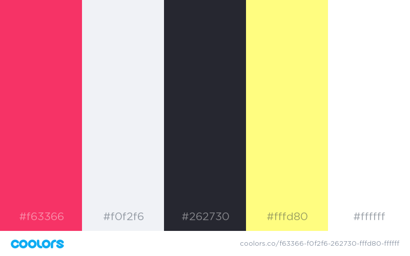
Main Colors

These colors are used throughout streamlit applications as of Feb 2, 2020.

Name	Hex	Use
Primary	`#f63366`	Primary pink/magenta used for widgets throughout the app
Secondary	`#f0f2f6`	Background color of Sidebar
Black	`#262730`	Font Color
Yellow (Light)	`#fffd80`	Right side of top header decoration in app
White	`#ffffff`	Background

View Colors

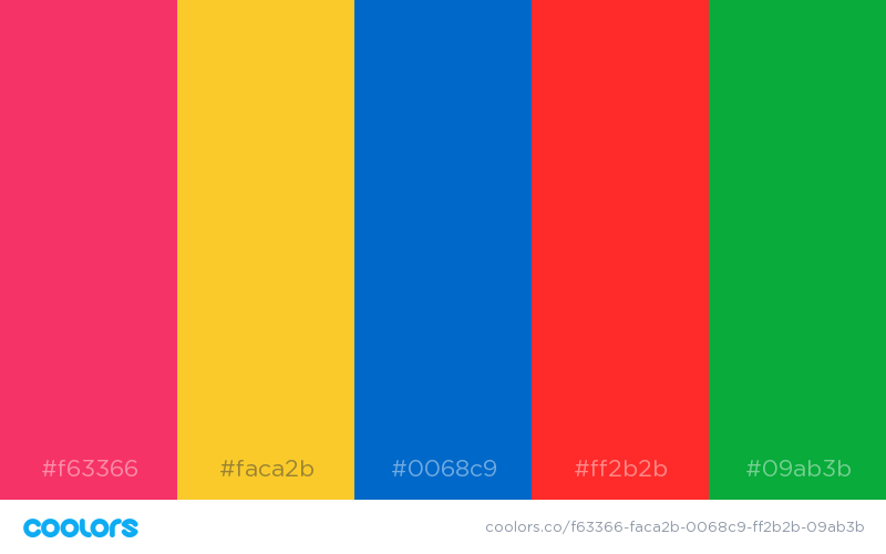
Other Secondary Colors

These are defined in the variables.scss file described below, but are not heavily used within the streamlit applications.

Name	Hex
Red	`#ff2b2b`
Yellow	`#faca2b`
Blue	`#0068c9`
Green	`#09ab3b`

View Colors

Fonts

Streamlit's default fonts are from the IBM Plex Collection

Text, including headers and markdown, is in IBM Plex Sans.

Code and data use IBM Plex Mono as the monospace font. This is used in markdown code blocks, the use of st.echo(), widget labels, st.json(), and rendered dataframes via st.dataframe and st.table.

Details

SCSS Variables

The essential aspects of streamlit's theme can be found in the variables.scss file in the frontend assets folder in the streamlit repository.

The essentials of the file are below (it's been slightly edited from the original file to remove extra information).

$gray-200: #f0f2f6;
$gray-600: #a3a8b4;
$gray-900: #262730;
$black: $gray-900;
$red: #ff2b2b;
$yellow: #faca2b;
$blue: #0068c9;
$green: #09ab3b;

$gray-lightest: $gray-200;
$yellow-light: #fffd80;

$primary: #f63366;
$secondary: $gray;

$font-family-sans-serif: "IBM Plex Sans", sans-serif;
$font-family-monospace: "IBM Plex Mono", monospace;

Bootstrap

Streamlit uses the Bootstrap framework behind the scenes. This means you can use bootstrap helper classes, for example img-fluid, if you're writing HTML within Markdown.

Generating New Palettes

If you want to generate some good looking color schemes that play off the existing streamlit colors, colormind.io and coolors.co are two helpful tools for creating new color schemes based off of a primary color. For generating color scales or palettes with more than 5 colors, the Chroma.js Color Palette Helper can't be beat.

Theme Essentials

Theme Essentials

Main Colors

These colors are used throughout streamlit applications as of Feb 2, 2020.

Name	Hex	Use
Primary	`#f63366`	Primary pink/magenta used for widgets throughout the app
Secondary	`#f0f2f6`	Background color of Sidebar
Black	`#262730`	Font Color
Yellow (Light)	`#fffd80`	Right side of top header decoration in app
White	`#ffffff`	Background

View Colors

Other Secondary Colors

These are defined in the variables.scss file described below, but are not heavily used within the streamlit applications.

Name	Hex
Red	`#ff2b2b`
Yellow	`#faca2b`
Blue	`#0068c9`
Green	`#09ab3b`

View Colors

Fonts

Streamlit's default fonts are from the IBM Plex Collection

Text, including headers and markdown, is in IBM Plex Sans.

Details

SCSS Variables

The essential aspects of streamlit's theme can be found in the variables.scss file in the frontend assets folder in the streamlit repository.

The essentials of the file are below (it's been slightly edited from the original file to remove extra information).

$gray-200: #f0f2f6;
$gray-600: #a3a8b4;
$gray-900: #262730;
$black: $gray-900;
$red: #ff2b2b;
$yellow: #faca2b;
$blue: #0068c9;
$green: #09ab3b;

$gray-lightest: $gray-200;
$yellow-light: #fffd80;

$primary: #f63366;
$secondary: $gray;

$font-family-sans-serif: "IBM Plex Sans", sans-serif;
$font-family-monospace: "IBM Plex Mono", monospace;

Bootstrap

Streamlit uses the Bootstrap framework behind the scenes. This means you can use bootstrap helper classes, for example img-fluid, if you're writing HTML within Markdown.

Generating New Palettes

Theming Altair

Theming Altair

Summary

If you use Altair for visualizations, you can define a custom theme to adjust the look of your visualization to match streamlit's theme.

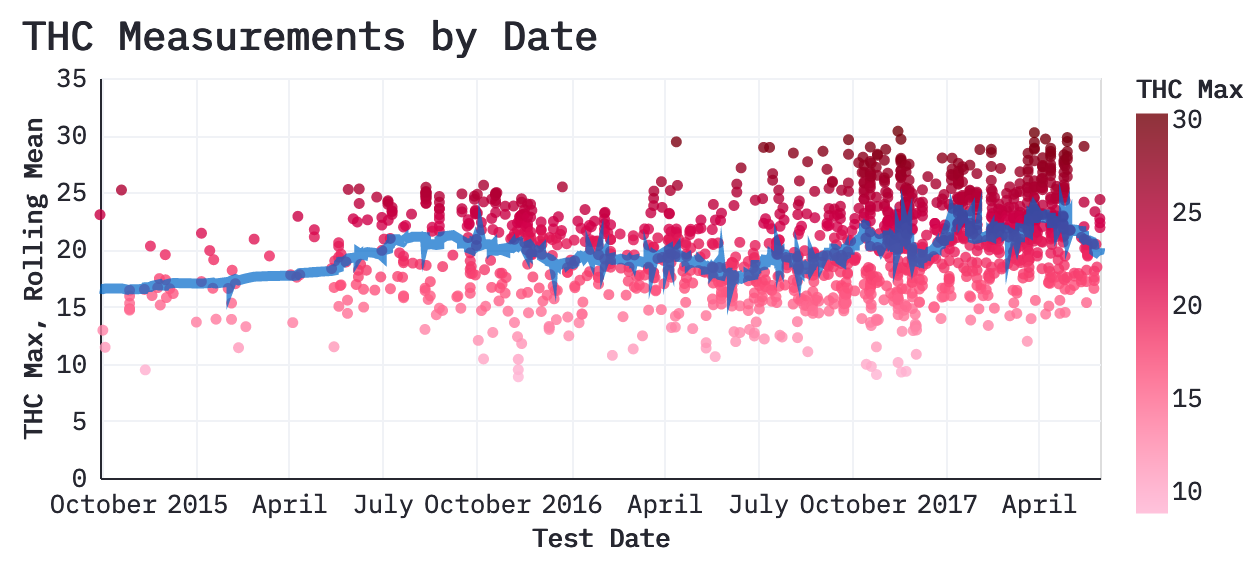
Streamlit Altair Theme

The python code below will apply a theme to your Altair visualizations that by default should match streamlit's theme settings. The default single color scale uses gradation of the primary color and was built with the Chroma.js Color Palette Helper. The divergent scale uses the primary color and the blue from the secondary colors. The categorical palette is a 5-color palette with the primary color, light-yellow secondary color, and remaining colors from the secondary palette.

The theme also adjusts the font to IBM Plex Mono to match data in dataframes and tables. It also adjusts the font sizes so that labels match the size of table elements and the chart title is the same size as an <h3> (header 3) element.

Example

Plot Example

Theme Code

def streamlit_theme():
    font = "IBM Plex Mono"
    primary_color = "#F63366"
    font_color = "#262730"
    grey_color = "#f0f2f6"
    base_size = 16
    lg_font = base_size * 1.25
    sm_font = base_size * 0.8  # st.table size
    xl_font = base_size * 1.75

    config = {
        "config": {
            "arc": {"fill": primary_color},
            "area": {"fill": primary_color},
            "circle": {"fill": primary_color, "stroke": font_color, "strokeWidth": 0.5},
            "line": {"stroke": primary_color},
            "path": {"stroke": primary_color},
            "point": {"stroke": primary_color},
            "rect": {"fill": primary_color},
            "shape": {"stroke": primary_color},
            "symbol": {"fill": primary_color},
            "title": {
                "font": font,
                "color": font_color,
                "fontSize": lg_font,
                "anchor": "start",
            },
            "axis": {
                "titleFont": font,
                "titleColor": font_color,
                "titleFontSize": sm_font,
                "labelFont": font,
                "labelColor": font_color,
                "labelFontSize": sm_font,
                "gridColor": grey_color,
                "domainColor": font_color,
                "tickColor": "#fff",
            },
            "header": {
                "labelFont": font,
                "titleFont": font,
                "labelFontSize": base_size,
                "titleFontSize": base_size,
            },
            "legend": {
                "titleFont": font,
                "titleColor": font_color,
                "titleFontSize": sm_font,
                "labelFont": font,
                "labelColor": font_color,
                "labelFontSize": sm_font,
            },
            "range": {
                "category": ["#f63366", "#fffd80", "#0068c9", "#ff2b2b", "#09ab3b"],
                "diverging": [
                    "#850018",
                    "#cd1549",
                    "#f6618d",
                    "#fbafc4",
                    "#f5f5f5",
                    "#93c5fe",
                    "#5091e6",
                    "#1d5ebd",
                    "#002f84",
                ],
                "heatmap": [
                    "#ffb5d4",
                    "#ff97b8",
                    "#ff7499",
                    "#fc4c78",
                    "#ec245f",
                    "#d2004b",
                    "#b10034",
                    "#91001f",
                    "#720008",
                ],
                "ramp": [
                    "#ffb5d4",
                    "#ff97b8",
                    "#ff7499",
                    "#fc4c78",
                    "#ec245f",
                    "#d2004b",
                    "#b10034",
                    "#91001f",
                    "#720008",
                ],
                "ordinal": [
                    "#ffb5d4",
                    "#ff97b8",
                    "#ff7499",
                    "#fc4c78",
                    "#ec245f",
                    "#d2004b",
                    "#b10034",
                    "#91001f",
                    "#720008",
                ],
            },
        }
    }
    return config

Applying the Theme

After you define this function, you'll need to register the theme with Altair wherever you define your plots.

alt.themes.register("streamlit", streamlit_theme)
alt.themes.enable("streamlit")

Alternative Theme

This alternative theme is closer to the default theme in ggplot2. It adds a grey background, changes the grid to white, and removes some of the dark plot spine.

Example

Alternative Theme

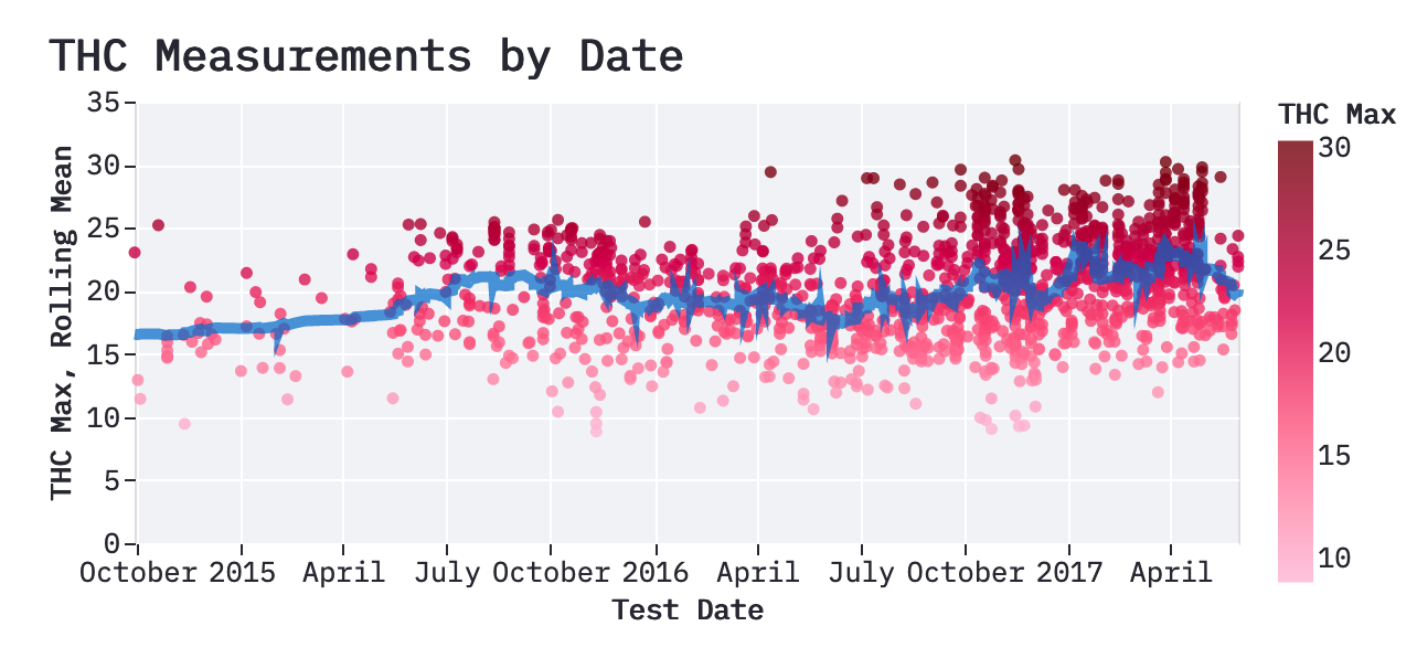
Theme Code

def streamlit_theme_alt():
    font = "IBM Plex Mono"
    primary_color = "#F63366"
    font_color = "#262730"
    grey_color = "#f0f2f6"
    base_size = 16
    lg_font = base_size * 1.25
    sm_font = base_size * 0.8  # st.table size
    xl_font = base_size * 1.75

    config = {
        "config": {
            "view": {"fill": grey_color},
            "arc": {"fill": primary_color},
            "area": {"fill": primary_color},
            "circle": {"fill": primary_color, "stroke": font_color, "strokeWidth": 0.5},
            "line": {"stroke": primary_color},
            "path": {"stroke": primary_color},
            "point": {"stroke": primary_color},
            "rect": {"fill": primary_color},
            "shape": {"stroke": primary_color},
            "symbol": {"fill": primary_color},
            "title": {
                "font": font,
                "color": font_color,
                "fontSize": lg_font,
                "anchor": "start",
            },
            "axis": {
                "titleFont": font,
                "titleColor": font_color,
                "titleFontSize": sm_font,
                "labelFont": font,
                "labelColor": font_color,
                "labelFontSize": sm_font,
                "grid": True,
                "gridColor": "#fff",
                "gridOpacity": 1,
                "domain": False,
                # "domainColor": font_color,
                "tickColor": font_color,
            },
            "header": {
                "labelFont": font,
                "titleFont": font,
                "labelFontSize": base_size,
                "titleFontSize": base_size,
            },
            "legend": {
                "titleFont": font,
                "titleColor": font_color,
                "titleFontSize": sm_font,
                "labelFont": font,
                "labelColor": font_color,
                "labelFontSize": sm_font,
            },
            "range": {
                "category": ["#f63366", "#fffd80", "#0068c9", "#ff2b2b", "#09ab3b"],
                "diverging": [
                    "#850018",
                    "#cd1549",
                    "#f6618d",
                    "#fbafc4",
                    "#f5f5f5",
                    "#93c5fe",
                    "#5091e6",
                    "#1d5ebd",
                    "#002f84",
                ],
                "heatmap": [
                    "#ffb5d4",
                    "#ff97b8",
                    "#ff7499",
                    "#fc4c78",
                    "#ec245f",
                    "#d2004b",
                    "#b10034",
                    "#91001f",
                    "#720008",
                ],
                "ramp": [
                    "#ffb5d4",
                    "#ff97b8",
                    "#ff7499",
                    "#fc4c78",
                    "#ec245f",
                    "#d2004b",
                    "#b10034",
                    "#91001f",
                    "#720008",
                ],
                "ordinal": [
                    "#ffb5d4",
                    "#ff97b8",
                    "#ff7499",
                    "#fc4c78",
                    "#ec245f",
                    "#d2004b",
                    "#b10034",
                    "#91001f",
                    "#720008",
                ],
            },
        }
    }
    return config

Again, be sure you register the theme after you define it. Note that this function is called streamlit_theme_alt.

Large Categorical Color Palette

The palette below may be helpful if you have more than 5 categories. It was generated by alternating colors on this divergent scale which uses some of the primary and secondary colors.

category_large = [
    "#f63366",
    "#0068c9",
    "#fffd80",
    "#7c61b0",
    "#ffd37b",
    "#ae5897",
    "#ffa774",
    "#d44a7e",
    "#fd756d",
]

Images

Images

Summary

Images can be used to flexibly add header content, additional instructions, brand logos, or other information about your app. I've found it easiest to design images for the default width of the main container and sidebar for an app viewed on desktop. Since I don't need to view these images fullscreen or use the in an interactive way throughout the app, I use a helper function to convert images to bytes and display them as HTML through a st.markdown, rather than using st.image. I'll cover all these steps below.

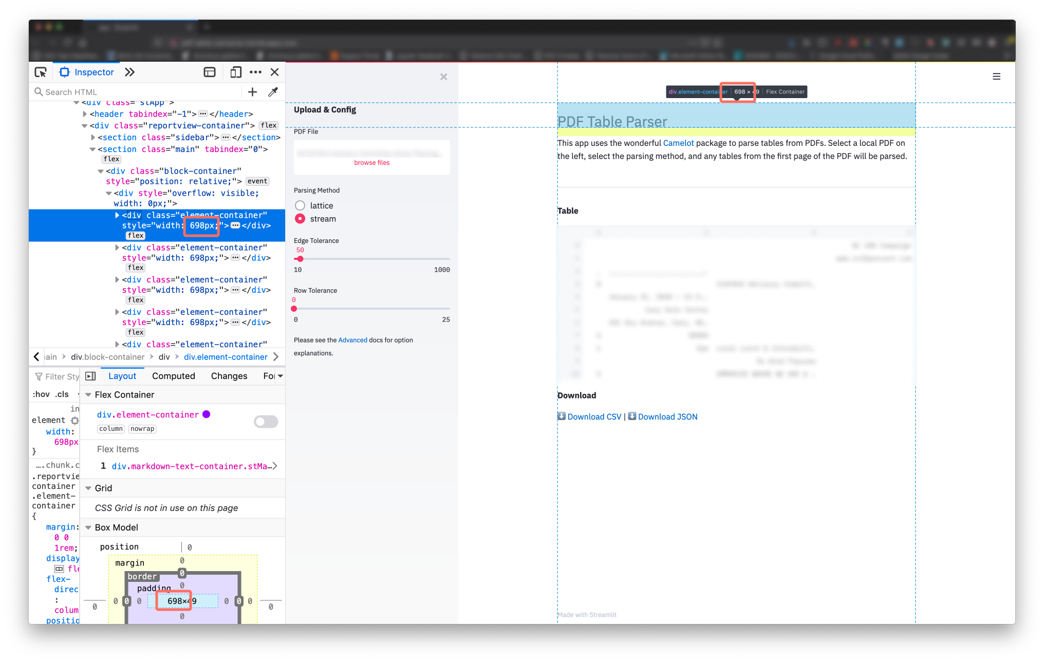
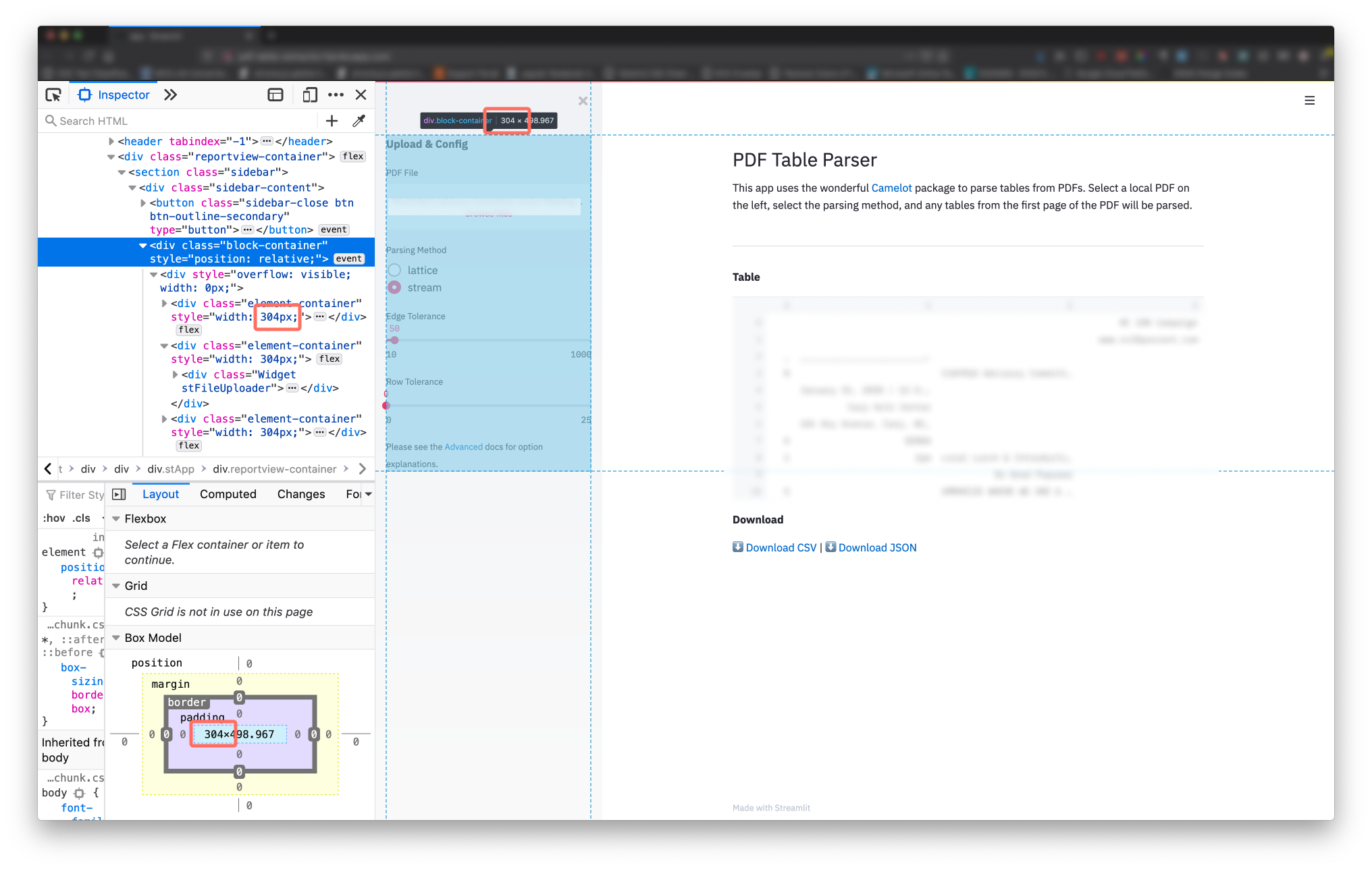
Container Sizes

As of Feb 2, 2020.

The main container content is 698px wide. The sidebar content is 304px wide.

Details

Images detailing how these numbers were determined are expandable below.

View Main Content Width Determination

View Sidebar Width Determination

Creating Header Images

One simple use case for images is a header image for your applications.

If you want to match the other content in your application, use the information from the Theme Essentials. You can download IBM Plex Sans and IBM Plex Mono from Google Fonts for local use.

The most staightforward way I've found to create header images, especially if they're mostly text, is to use Figma. Figma is a tool typically used for designing interfaces, but I typically use it for more lightweight design tasks like creating simple image assets. As a plus, Figma is really easy to learn and has a relatively simple interface.

Using Figma

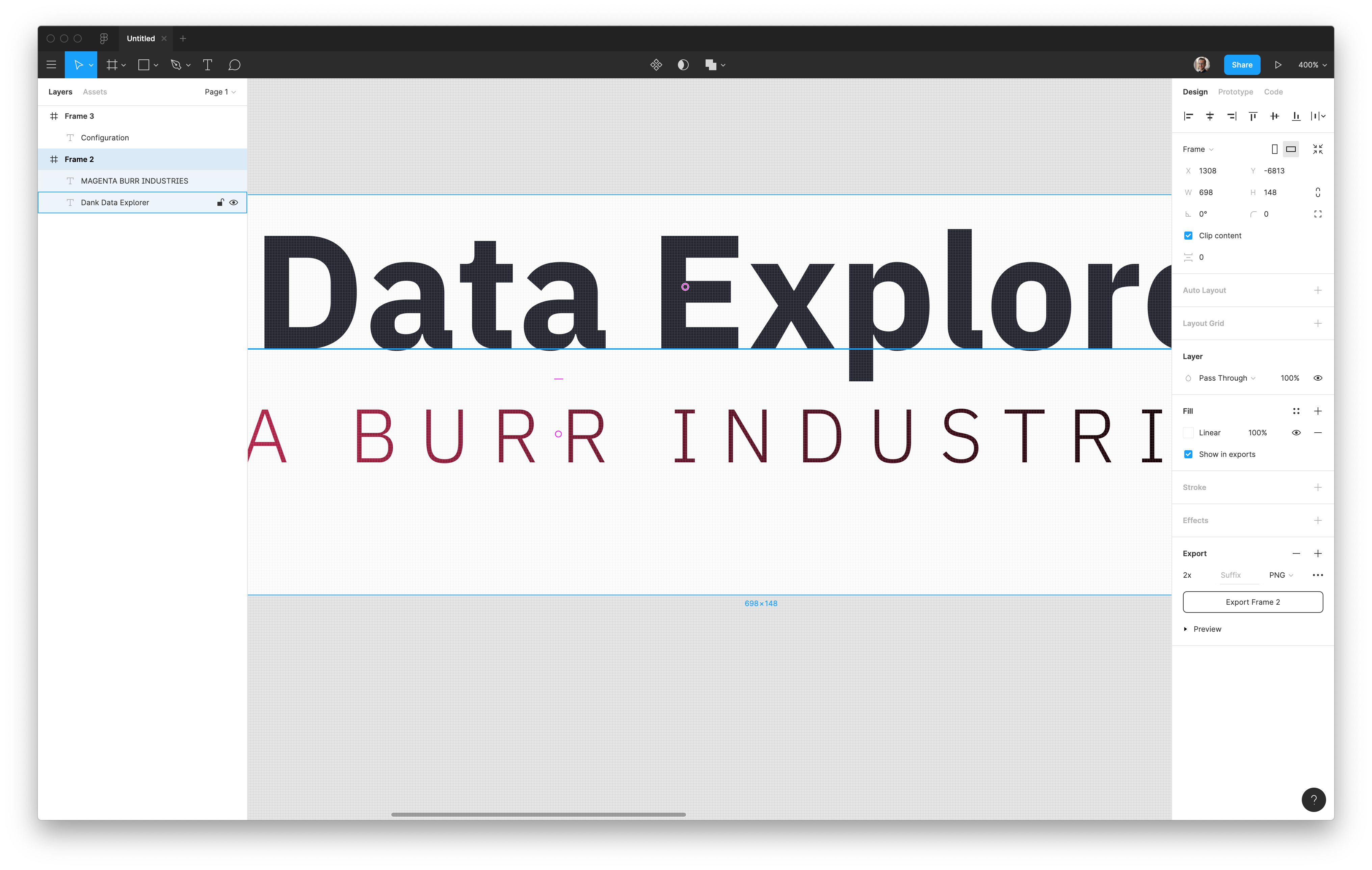
First, use the Frame tool to create a frame. This is a container for your image. Create the frame so it has a width of the streamlit container where it will be placed. You can adjust the height so it makes sense for your content.
Design to your heart's content. Start simple by using IBM Plex Sans as your font and the standard streamlit colors. Some simple elements to play around with are character spacing, all caps, and gradient scaling your text.
Once you're finished, select your Frame then use the Export menu in the lower right to export your image to your streamlit app directory.

Displaying Your Image in App

Since I don't need any interaction with the image, I display the HTML through st.markdown rather than st.image.

We'll convert the image to bytes so that it can be displayed using an <img> HTML element. The helper function below takes the path to the image (from your app.py) and converts it to bytes.

def img_to_bytes(img_path):
    img_bytes = Path(img_path).read_bytes()
    encoded = base64.b64encode(img_bytes).decode()
    return encoded

From there, you can use the image in your app as follows:

header_html = "<img src='data:image/png;base64,{}' class='img-fluid'>".format(
    img_to_bytes("header.png")
)
st.markdown(
    header_html, unsafe_allow_html=True,
)

Streamlit uses bootstrap, so we can take advantage of the img-fluid class to make sure that the image is responsive as the app is resized.

Markdown

Markdown

Summary

Markdown has several uses within a streamlit application. As the only tool for custom HTML within a streamlit app, you can use it to flexibly insert rich content into your application.

Using Markdown Files

If you have content beyond a sentence in length or want an easier way to write multi-line markdown content, create a separate markdown file and import that content into your app where needed.

For example, your app might have some introductory text. Create an introduction.md file and write in there, then import the content into a markdown widget.

from pathlib import Path
import streamlit as st

def read_markdown_file(markdown_file):
    return Path(markdown_file).read_text()

intro_markdown = read_markdown_file("introduction.md")
st.markdown(intro_markdown, unsafe_allow_html=True)

Conditionally Displaying Long Content

If you use the method above to write and display long markdown content, you might not want to always have the content displayed since it takes up a significant portion of the app's screen real estate. There are two options.

Hide it with a `st.checkbox`

In this example, let's say there's a data dictionary in data_dictionary.md. We can then use a st.checkbox to display this content somewhere when the checkbox is checked.

dict_check = st.checkbox("Data Dictionary")
dict_markdown = read_markdown_file("data_dictionary.md")

if dict_check:
    st.markdown(dict_markdown, unsafe_allow_html=True)

Use `<details><summary>` Elements in Markdown

Since you can use HTML in markdown, you can take advantage of the <details> element. Rather than using a streamlit widget, you "write" the widget using these elements in markdown.

For example, in a data_dictionary.md file, you would do the following:

<details>
<summary>Data Dictionary</summary>

## Data Dictionary

- Variable 1: this is variable 1
- Variable 2: this is variable 2
...

</details>

Remember that this will require you to pass unsafe_allow_html=True into st.markdown.

Use `<small>` Elements

If you have some disclaimer text that you want to display with a smaller font size, wrap it with a <small> tag within your markdown. The interaction with markdown and <small> is a little tricky. You'll likely have to wrap each markdown element (i.e. paragraph, single bullet, etc.) with the tag -- not just put the tag around everything you'd like to be small.

Remember that this will require you to pass unsafe_allow_html=True into st.markdown.

Use `st.markdown("---")` for Visual Separation

In markdown, --- will create a horizontal rule <hr> element. These can be helpful to section your application. For example in the Dank Data Explorer the app is sectioned into 4 distinct parts: the sidebar configuration options, the app details, the header of the app, and the body of the app.

Sectioning with ---

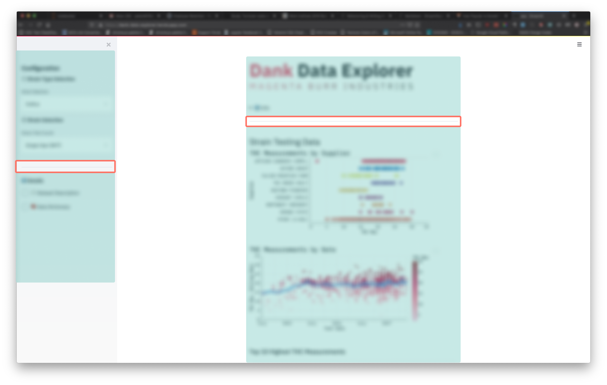
Sections of app in blue, <hr> elements surrounded by orange.

Don't Forget Emoji

Emoji can serve as little icons to highlight certain functionality of your app. For example, ℹ️ can be used to indicate contextual information, or ✅ and 🚫 can be used for positive and negative examples.

There are also several styles of emoji numerials (① ⑴ ⓵ ❶) that can be used to guide a user through the sequence of options within your app.

Combine f-strings with Markdown

In building an interface around an analysis, much of it requires creating or manipulating strings in variable names, widget values, axis labels, widget labels, or narrative description.

If we want to display some analysis in narrative form and there’s a few particular variables we want to highlight, f-strings and markdown can help us out. Beyond an easy way to fill strings with specific variable values, it’s also an easy way to format them inline. For example, we might use something like this to display basic info about a column in a dataset and highlight them in a markdown string.

mean = df["values"].mean()
n_rows = len(df)

md_results = f"The mean is **{mean:.2f}** and there are **{n_rows:,}**."

st.markdown(md_results)

We’ve used two formats here: .2f to round a float to two decimal places and , to use a comma as a thousands separator. We've also used markdown syntax to bold the values so that they're visually prominent in the text.

Markdown

Markdown

Summary

Markdown has several uses within a streamlit application. As the only tool for custom HTML within a streamlit app, you can use it to flexibly insert rich content into your application.

Using Markdown Files

If you have content beyond a sentence in length or want an easier way to write multi-line markdown content, create a separate markdown file and import that content into your app where needed.

For example, your app might have some introductory text. Create an introduction.md file and write in there, then import the content into a markdown widget.

from pathlib import Path
import streamlit as st

def read_markdown_file(markdown_file):
    return Path(markdown_file).read_text()

intro_markdown = read_markdown_file("introduction.md")
st.markdown(intro_markdown, unsafe_allow_html=True)

Conditionally Displaying Long Content

Hide it with a `st.checkbox`

In this example, let's say there's a data dictionary in data_dictionary.md. We can then use a st.checkbox to display this content somewhere when the checkbox is checked.

dict_check = st.checkbox("Data Dictionary")
dict_markdown = read_markdown_file("data_dictionary.md")

if dict_check:
    st.markdown(dict_markdown, unsafe_allow_html=True)

Use `<details><summary>` Elements in Markdown

Since you can use HTML in markdown, you can take advantage of the <details> element. Rather than using a streamlit widget, you "write" the widget using these elements in markdown.

For example, in a data_dictionary.md file, you would do the following:

<details>
<summary>Data Dictionary</summary>

## Data Dictionary

- Variable 1: this is variable 1
- Variable 2: this is variable 2
...

</details>

Remember that this will require you to pass unsafe_allow_html=True into st.markdown.

Use `<small>` Elements

Remember that this will require you to pass unsafe_allow_html=True into st.markdown.

Use `st.markdown("---")` for Visual Separation

Sectioning with ---

Sections of app in blue, <hr> elements surrounded by orange.

Don't Forget Emoji

There are also several styles of emoji numerials (① ⑴ ⓵ ❶) that can be used to guide a user through the sequence of options within your app.

Combine f-strings with Markdown

In building an interface around an analysis, much of it requires creating or manipulating strings in variable names, widget values, axis labels, widget labels, or narrative description.

mean = df["values"].mean()
n_rows = len(df)

md_results = f"The mean is **{mean:.2f}** and there are **{n_rows:,}**."

st.markdown(md_results)

Display Clean Variable Names

The variable names in a DataFrame might be snake cased or formatted in a way not appropriate for end users, e.g. pointless_metric_my_boss_requested_and_i_reluctantly_included. Most of the streamlit widgets contain a format_func parameter which takes function that applies formatting for display to the option values you provide the widget. As a simple example, you could title case each of the variable names.

You can also use this functionality, combined with a dictionary, to explicitly handle the formatting of your values. The example below cleans up the column names from the birdstrikes dataset for use as a dropdown to describe each column.

import streamlit as st
from vega_datasets import data


@st.cache
def load_data():
    return data.birdstrikes()


cols = {
    "Airport__Name": "Airport Name",
    "Aircraft__Make_Model": "Aircraft Make & Model",
    "Effect__Amount_of_damage": "Effect: Amount of Damage",
    "Flight_Date": "Flight Date",
    "Aircraft__Airline_Operator": "Airline Operator",
    "Origin_State": "Origin State",
    "When__Phase_of_flight": "When (Phase of Flight)",
    "Wildlife__Size": "Wildlife Size",
    "Wildlife__Species": "Wildlife Species",
    "When__Time_of_day": "When (Time of Day)",
    "Cost__Other": "Cost (Other)",
    "Cost__Repair": "Cost (Repair)",
    "Cost__Total_$": "Cost (Total) ($)",
    "Speed_IAS_in_knots": "Speed (in Knots)",
}

dataset = load_data()

column = st.selectbox("Describe Column", list(dataset.columns), format_func=cols.get)

st.write(dataset[column].describe())

Link to Gist

Use Caching (and Benchmark It)

It can be tempting to throw that handy @st.cache decorator on everything and hope for the best. However, mindlessly applying caching means that we're missing a great opportunity to get meta and use streamlit to understand where caching helps the most.

Rather than decorating every function, create two versions of each function: one with the decorator and one without. Then do some basic benchmarking of how long it takes to execute both the cached and uncached versions of that function.

In the example below, we simulate loading a large dataset by concatenating 100 copies of the airports dataset, then dynamically selecting the first n rows and describing them.

import streamlit as st
from vega_datasets import data
from time import time
import pandas as pd


@st.cache
def load_data():
    return pd.concat((data.airports() for _ in range(100)))


@st.cache
def select_rows(dataset, nrows):
    return dataset.head(nrows)


@st.cache
def describe(dataset):
    return dataset.describe()


rows = st.slider("Rows", min_value=100, max_value=3300 * 100, step=10000)

start_uncached = time()
dataset_uncached = pd.concat((data.airports() for _ in range(100)))
load_uncached = time()
dataset_sample_uncached = dataset_uncached.head(rows)
select_uncached = time()
describe_uncached_dataset = dataset_sample_uncached.describe()
finish_uncached = time()
benchmark_uncached = (
    f"Cached. Total: {finish_uncached - start_uncached:.2f}s"
    f" Load: {load_uncached - start_uncached:.2f}"
    f" Select: {select_uncached - load_uncached:.2f}"
    f" Describe: {finish_uncached - select_uncached:.2f}"
)

st.text(benchmark_uncached)
st.write(describe_uncached_dataset)

start_cached = time()
dataset_cached = load_data()
load_cached = time()
dataset_sample_cached = select_rows(dataset_cached, rows)
select_cached = time()
describe_cached_dataset = describe(dataset_sample_cached)
finish_cached = time()

benchmark_cached = (
    f"Cached. Total: {finish_cached - start_cached:.2f}s"
    f" Load: {load_cached - start_cached:.2f}"
    f" Select: {select_cached - load_cached:.2f}"
    f" Describe: {finish_cached - select_cached:.2f}"
)
st.text(benchmark_cached)
st.write(describe_cached_dataset)

Link to Gist

Since each step (data load, select rows, describe selection) of this is timed, we can see where caching provides a speedup. From my experience with this example, my heuristics for caching are:

Always cache loading the dataset
Probably cache functions that take longer than a half second
Benchmark everything else

I think caching is one of streamlit’s killer features and I know they’re focusing on it and improving it. Caching intelligently is also complex problem, so it’s a good idea to lean more towards benchmarking and validating that the caching functionality is acting as expected.

Create Dynamic Widgets

Many examples focus on creating dynamic visualizations, but don’t forget you can also program dynamic widgets. The simplest example of this need is when two columns in a dataset have a nested relationship and there are two widgets to select values from those two columns. When building an app to filter data, the the dropdown for the first column should change the options available in the second dropdown.

Linking behavior of two dropdowns is a common use case. The example below builds a scatterplot with the cars dataset. We need a dynamic dropdown here because the variable we select for the x-axis doesn't need to be available for selection in the y-axis.

We can also go beyond this basic dynamic functionality: what if we sorted the available y-axis options by their correlation with the selected x variable? We can calculate the correlations and combining this with the widget’s format_func to display variables and their correlations in sorted order.

import altair as alt
import streamlit as st
from vega_datasets import data

cars = data.cars()

quantitative_variables = [
    "Miles_per_Gallon",
    "Cylinders",
    "Displacement",
    "Horsepower",
    "Weight_in_lbs",
    "Acceleration",
]


@st.cache
def get_y_vars(dataset, x, variables):
    corrs = dataset.corr()[x]
    remaining_variables = [v for v in variables if v != x]
    sorted_remaining_variables = sorted(
        remaining_variables, key=lambda v: corrs[v], reverse=True
    )
    format_dict = {v: f"{v} ({corrs[v]:.2f})" for v in sorted_remaining_variables}
    return sorted_remaining_variables, format_dict


st.header("Cars Dataset - Correlation Dynamic Dropdown")
x = st.selectbox("x", quantitative_variables)
y_options, y_formats = get_y_vars(cars, x, quantitative_variables)
y = st.selectbox(
    f"y (sorted by correlation with {x})", y_options, format_func=y_formats.get
)

plot = alt.Chart(cars).mark_circle().encode(x=x, y=y)

st.altair_chart(plot)

Link to Gist

Altair for Visualizations

If you’ve been prototyping visualizations with another library, consider switching to Altair to build your visualizations. In my experience, I think there are three key reasons a switch could be beneficial:

Altair is probably faster (unless we’re plotting a lot of data)
It operates directly on pandas DataFrames
Interactive visualizations are easy to create

On the first point about speed, we can see a drastic speedup if we prototyped using matplotlib. Most of that speedup is just the fact that it takes more time to render a static image and place it in the app compared to rendering a javascript visualization. This is demonstrated in the example app below, which generates a scatterplot for some generated data and outputs the timing for the creation and rendering for each part of the visualization.

from time import time

import altair as alt
import matplotlib.pyplot as plt
import numpy as np
import pandas as pd
import streamlit as st


def mpl_scatter(dataset, x, y):
    fig, ax = plt.subplots()
    dataset.plot.scatter(x=x, y=y, alpha=0.8, ax=ax)
    return fig


def altair_scatter(dataset, x, y):
    plot = (
        alt.Chart(dataset, height=400, width=400)
        .mark_point(filled=True, opacity=0.8)
        .encode(x=x, y=y)
    )
    return plot


size = st.slider("Size", min_value=1000, max_value=100_000, step=10_000)
dataset = pd.DataFrame(
    {"x": np.random.normal(size=size), "y": np.random.normal(size=size)}
)

mpl_start = time()
mpl_plot = mpl_scatter(dataset, "x", "y")
mpl_finish = time()

st.pyplot(mpl_plot)
mpl_render = time()
st.subheader("Matplotlib")
st.write(f"Create: {mpl_finish - mpl_start:.3f}s")
st.write(f"Render: {mpl_render - mpl_finish:.3f}s")
st.write(f"Total: {mpl_render - mpl_start:.3f}s")

alt_start = time()
alt_plot = altair_scatter(dataset, "x", "y")
alt_finish = time()

st.altair_chart(alt_plot)
alt_render = time()
st.subheader("Altair")
st.write(f"Create: {alt_finish - alt_start:.3f}s")
st.write(f"Render: {alt_render - alt_finish:.3f}s")
st.write(f"Total: {alt_render - alt_start:.3f}s")

speedup = (mpl_render - mpl_start) / (alt_render - alt_start)
st.write(f"MPL / Altair Ratio: {speedup:.1f}x")

Link to Gist

Working directly with DataFrames provides another benefit. It can ease the debugging process: if there’s an issue with the input data, we can use st.write(df) to display the DataFrame in a streamlit app and inspect it. This makes the feedback loop for debugging data issues much shorter. The second benefit is that it reduces the amount of transformational glue code sometimes required to create specific visualizations. For basic plots, we could use a DataFrame's plotting methods, but more complex visualizations might require us to restructure our dataset in a way that makes sense with the visualization API. This additional code between the dataset and visualization can be the source of additional complexity and can be a pain point as the app grows. Since Altair uses the Vega-Lite visualization grammar, the functions available in the transforms API can be used to make any visualization appropriate transformations.

Finally, interactive visualizations with Altair are easy. While an app might start by using streamlit widgets to filter and select data, an app could also use a visualization could as the selection mechanism. Rather than communicating information as a string in a widget or narrative, (interactive visualizations)[https://altair-viz.github.io/gallery/index.html#interactive-charts] allow visual communication of aspects of the data within a visualization.

Refactoring & Writing Modular Code

It’s easy to spend a few hours with streamlit and have a 500 line app.py file that nobody but you understands. If you're handing off your code, deploying your app, or adding a some new functionality it's now possible that you'll be spending a significant amount of time trying to remember how your code works because you've neglected good code hygiene.

If an app is beyond 100 lines of code, it can probably benefit from a refactor. A good first step is to create functions from the code and put those functions in a separate helpers.py file. This also makes it easier to test and benchmark caching on these functions.

There’s no specific right way on how exactly to refactor code, but I’ve developed an exercise that can help when starting an app refactor.

Refactoring Exercise

In the app.py, try to:

only import streamlit and helper functions (don’t forget to benchmark @st.cache on these helper functions)
never create a variable that isn’t input into a streamlit object, i.e. visualization or widget, in the next line of code (with the exception of the data loading function)

These aren’t hard and fast rules to always abide by: you could follow them specifically and have a poorly organized app because you’ve got large, complex functions that do too much. However, they are good objectives to start with when moving from everything in app.py to a more modular structure. The example below highlights an app before and after going through this exercise.

⛔️ BAD EXAMPLE: PRE-REFACTOR

# app.py
import streamlit as st
import pandas as pd

data = pd.read_csv("data.csv")  # no function → no cache, requires pandas import: 👎,👎
sample = data.head(100)  # not input into streamlit object: 👎
described_sample = sample.describe()  # input into streamlit object: ✅
st.write(described_sample)

✅ GOOD EXAMPLE

# app.py
import streamlit as st
from helpers import load_data, describe_sample

data = load_data()  # data import: ✅
described_sample = describe_sample(data, 100)  # input into streamlit object: ✅
st.write(described_sample)

# helpers.py
import streamlit as st
import pandas as pd


@st.cache
def load_data():
    return pd.read_csv("data.csv")


@st.cache
def describe_sample(dataset, nrows):
    sample = dataset.head(nrows)
    return sample.describe()

Another benefit of reorganizing code in this way is that the functions in the helpers file are now easier to write tests for. Sometimes I struggle with coming up with ideas of what to test, but I’ve found that now it’s really easy to come up with tests for my apps because I’m more quickly discovering bugs and edge cases now that I’m interacting more closely with the data and code. Now, any time my app displays a traceback, I fix the function that caused it and write a test to make sure the new behavior is what I expect.

Example Apps

Gists

The following apps are gists, which you can run directly with streamlit installed by running streamlit run <GIST URL>

Full Apps

Dank Data Explorer
- 💡 This app was created to serve as an example of many of the Design and Markdown ideas.
Spotify Track Orderer
PDF Table Extractor
Distribution Fitter

Awesome-Streamlit contains many more examples of streamlit apps.

Appendix

Build Process

This documentation is built using the wonderful Rust package mdBook.

The build process is automated using GitHub Actions to host it on GitHub Pages, with the GitHub Pages Action and the mdBook Action.

Streamlitopedia